Overview of LETSmix

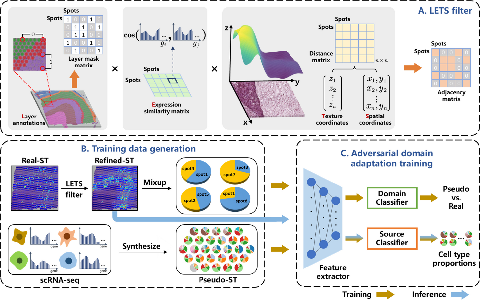
The proposed cell-type deconvolution method integrates spatial correlations among spots while eliminating domain variances between the ST and the reference scRNA-seq data. As illustrated in Fig. 1, both the scRNA-seq and ST data were preprocessed before they were fed into the deep learning network. The synthesis of pseudo-ST from annotated scRNA-seq data was implemented by randomly selecting cells to generate pseudo-spots, with their total gene expression counts determined by a weighted sum of the chosen cells. This procedure accumulated a substantial corpus of pseudo-ST data with known cell type compositions, facilitating supervised training of the feature extractor and source classifier. Real-ST data were locally smoothed with ancillary spatial context information. Considering potential noise in expression data due to limited cell numbers per spot and sequencing techniques, it is rational to aggregate information from neighboring spots with similar histological and gene expression features [32]. To this end, an adjacency matrix, termed the LETS filter, was designed to signify spatial, histological, and gene expression similarities among real-ST spots. Further optimization of this matrix incorporated layer annotations as masks, restricting information sharing to spots within the same layer. Multiplying the constructed adjacency matrix with the original real-ST expression count matrix effectively enhances the data quality. Due to inherent technical differences between ST and scRNA-seq, the refined real-ST and synthetic pseudo-ST data underwent adversarial training within the deep learning network, employing a label inversion technique commonly used in domain adaptation methods. This technique ensures that the learned domain classifier effectively distinguishes real-spots from pseudo-spots, while the extracted features try to deceive the trained domain classifier. Notably, augmented training data were generated by mixing spots randomly selected from the spatially refined real-ST data to compensate for the significant disparity in data volume between real-spots and pseudo-spots. Thus, the source classifier, trained exclusively with labeled pseudo-ST, demonstrates superior performance in estimating cell type compositions from real-ST data.

To assess the efficacy of our proposed deconvolution method, LETSmix was applied to four representative public real ST datasets (Additional file 1: Table S3). These datasets encompass 12 ST samples of human brain cortex (DLPFC) data, 2 ST samples of human pancreatic ductal adenocarcinoma (PDAC) data, 3 ST samples of mouse liver (Liver) data, and 1 ST sample of Mouse olfactory bulb (MOB) data. All the ST samples in the DLPFC dataset share a common reference scRNA-seq dataset, while each PDAC ST sample is paired with a matched reference scRNA-seq dataset, supplemented by an external scRNA-seq dataset. The Liver dataset comprises 3 distinct scRNA-seq datasets with different sequencing protocols, and only one scRNA-seq dataset is used to deconvolve MOB ST data. The performance of LETSmix was benchmarked against that of other state-of-the-art methods, including CellDART, SpaDecon, Cell2location, POLARIS, and CARD, through qualitative heuristic inspection and quantitative evaluation using metrics such as Area Under the Curve (AUC), EnRichment (ER), Jensen-Shannon Divergence (JSD), and Moran’s I. Among these metrics, the AUC and ER evaluate the enrichment of regionally restricted cell types within target areas, while the JSD measures the consistency of the overall cell-type proportions between the entire ST tissue region and the matched reference scRNA-seq dataset. Moran’s I assesses the spatial autocorrelation of cell type distributions, indicating whether specific cell types exhibit clustered or dispersed spatial patterns.

Benchmarking and robustness evaluation of LETSmix in deconvolution of human DLPFC data

We assessed the performance of LETSmix using a 10X Visium dataset derived from postmortem neurotypical human DLPFC tissues [38]. In this dataset, 12 ST samples exhibit clear structural stratification, ranging from L1 to L6 and WM (white matter) annotated by pathologists (Fig. 2A, Additional file 1: Fig. S2). A shared reference scRNA-seq dataset [14] was applied to train each deconvolution method for benchmarking, as visualized by the UMAP representation in Fig. 2B. Among the 28 annotated cell types, the spatial mapping results of 10 layer-specific excitatory neurons were used to quantify the deconvolution performance of the different tools.

Fig. 2

Application to the human brain cortex 10X Visium dataset. A Layer annotations of the ST sample named “151,673” in the DLPFC dataset. B UMAP representation of the reference scRNA-seq dataset. C Box plots displaying the calculated AUC and ER values for the estimated cell type distribution in all 12 ST samples. Each box comprises 50 datapoints that represent scores for 10 layer-specific cell types in 5 repeated experiments, and ranges from the third and first quartiles with the median as the horizontal line, while whiskers represent 1.5 times the interquartile range from the lower and upper bounds of the box. D Estimated proportion heatmaps of 3 layer-specific excitatory neurons by each deconvolution method. E Box plots showing the calculated AUC and ER values for the estimated cell type distributions in the “151,673” ST sample. “original” includes all 28 cell types in the scRNA-seq dataset. “merge” indicates that the cell subtypes were merged before model training except for the 10 excitatory neurons. “del Inhib” indicates that inhibitory neurons were deleted from the scRNA-seq dataset. F UMAP representation of deconvolution results from different methods under the “original” and “del Inhib” conditions. G Scatter plots of cluster centroid distances in the UMAP computed for each method under different condition pairs. H Clustering results of the “151,673” ST sample given by GraphST. I Ablation study on the “151,673” ST sample. “cluster” represents the situation where LETSmix leverages clustering results given by GraphST as the layer annotation information. “wo_LETS” represents the situation where LETSmix ignores all spatial context information, and “wo_DA” represents the situation where LETSmix is trained without the implementation of the domain adaptation strategy. Error bars represent the mean ± standard deviation. An independent t-test was performed between LETSmix and the other ablated models. Statistical significance is indicated above the bars (ns: not significant, ****P-value < 0.0001)

Figure 2C presents the box plots of the AUC and ER values achieved by different models on all 12 ST samples. The ranks of all these models remain consistent across the two metrics, with LETSmix consistently holding the top position. Due to the greater sensitivity of the AUC metric compared to that of the ER metric, the evaluation results based on the AUC metric exhibit more pronounced differences in cell-type deconvolution performances across different models. Figure 2D and Additional file 1: Fig. S3 show the spatial distribution heatmaps of layer-specific cell types estimated by each model trained exclusively on the ST sample named “151,673.” Compared to layer annotations, estimations of excitatory neurons from LETSmix were more accurate and coherent than those from other models. All excitatory neuron cell types estimated by LETSmix demonstrated reasonable regionally restricted patterns. For example, a distinct gap between layers 4 and 6 can be clearly observed in the LETSmix predictions for Ex_6_L4_6 cells. In contrast, the estimation results from other models were either excessively sparse or entirely fail to identify this cell type. Additionally, only LETSmix demonstrated the ability to correctly predict significantly more Ex_3_L4_5 cells within layers 4 and 5. Compared to CellDART, LETSmix exhibited a more continuous spatial distribution and fewer false positive results, crediting it to the utilization of information from spatial context. SpaDecon struggled to accurately predict the distribution of these cell types, mainly due to its neglect of the domain differences between the scRNA-seq and ST data during the modelling process. The same issue was also present in the CARD model. Although Cell2location also considered the domain shifts between data from the two sequencing technologies through traditional statistical probabilistic approaches, its performance fell short compared to that of the deep learning-based domain adaptation method employed in this study. Layer annotation information was also incorporated in POLARIS, but its estimation results evidently diffused into other non-target regions. Although GraphST and SpatialPrompt demonstrate a discernible stratification pattern in the deconvolution results for those excitatory neurons, substantial discrepancies persist when compared with the layer annotations. Additional file 1: Fig. S4 provides the results of all cell types estimated by LETSmix. Regarding other nonneuronal cells, LETSmix predicted that astrocytes are primarily distributed in layers 1 and 6, while oligodendrocytes were mainly located in the white matter region, which was consistent with findings from other biomedical studies [33], demonstrating the credibility and reliability of the predictions made by LETSmix.

Furthermore, LETSmix and other models were tested under three different conditions on the “151,673” ST sample. The AUC and ER values were calculated for each excitatory neuron type in 5 repeated experiments. As shown in Fig. 2E and Additional file 1: Fig. S5, the scRNA-seq dataset was used with the original 28 cell types for model training under the “original” condition. These 28 cell types include several cell subtypes. In the “merge” condition, these subtypes were merged into a broader category before training the models. For example, Astros_1, Astros_2, and Astros_3 were merged into the Astros cell type. Only the 10 layer-specific excitatory neuronal cell subtypes used for metric calculations were not merged, resulting in 16 cell types in total. Under the “del Inhib” condition, all cells belonging to the inhibitory subtype, which accounts for approximately 20% of the entire dataset, were removed from the scRNA-seq data before model training. For both metrics and three conditions, LETSmix consistently achieved the highest scores, evidently outperforming other models, in accordance with the visual inspection in Fig. 2D. To assess the robustness of different models under varying conditions, we visualized the predicted cell-type proportions of the ten neuronal cell types using UMAP representations, and further quantified the centroid distances in UMAP space between estimation results across different condition pairs for each method (Fig. 2F, G, and Additional file 1: Fig. S6). Interestingly, the traditional machine learning-based methods (Cell2location, POLARIS, CARD, and SpatialPrompt) demonstrated consistently higher stability when compared to most deep learning-based approaches (LETSmix, CellDART, and SpaDecon). This enhanced stability may be attributed to the handcrafted features and fewer variable parameters in traditional machine learning models, which are less prone to overfitting under varying conditions. However, among the deep learning models, LETSmix exhibited smaller centroid distances overall, second only to GraphST, indicating better consistency across different conditions. Despite the superior stability of machine learning-based methods and GraphST, they significantly lagged behind LETSmix in deconvolution accuracy. As a result, the apparent robustness of these methods is of limited utility, as their lower prediction accuracy undermines their practical relevance in accurately resolving cell type compositions from spatial transcriptomics data.

In real-world applications, it is often challenging to obtain precisely annotated spatial regions from expert pathologists due to the scarcity or inaccessibility of such detailed annotations for tissue samples. However, with the rapid advancement of clustering methodologies applied to omics data, automated spatial region annotation has become increasingly feasible through the use of sophisticated computational tools [34, 45, 46]. To explore this possibility, we evaluated the performance of LETSmix when employing clustering-based annotations, generated by GraphST, as a surrogate for expert-curated spatial regions in sample 151,673 (Additional file 1: Fig. S7). The clustering-based annotations achieved an Adjusted Rand Index (ARI) score of 0.63 when compared to the ground truth annotations (Fig. 2H), indicating a moderate level of agreement. To further assess the impact of this automated annotation approach on deconvolution performance, we compared results from LETSmix using the clustering-derived regions against the results obtained with expert annotations. Based on the AUC metric, no significant differences were observed between the two conditions (Fig. 2I), supporting the feasibility of using clustering-derived annotations for deconvolution tasks. This finding underscores the potential of automated computational methods in addressing the limitations posed by the lack of expert annotations, especially in large-scale spatial transcriptomics studies. In addition to the clustering-based evaluation, we further tested performance of LETSmix when spatial contextual information and domain adaptation were systematically omitted. Both modifications led to a marked decline in performance, highlighting the critical importance of these components in maintaining the robustness and accuracy of the deconvolution process.

LETSmix achieved superior and robust performance on PDAC data under matched and unmatched conditions

The second dataset used for evaluation originated from cancerous tissues from human PDAC patients. Here, ST and paired scRNA-seq data were collected following different protocols compared to those in the previously analyzed DLPFC dataset. We first applied LETSmix to an ST sample denoted as PDAC-A using paired scRNA-seq data for model training. The ST sample was delineated into four distinct regions by pathological experts (Fig. 3A). Among the annotated cell types in scRNA-seq (Fig. 3B), acinar, cancer, and ductal cells are expected to be located within specific regions (Additional file 1: Table S1). As previously discussed in the “Evaluation metrics” section, the AUC metric presents certain limitations when assessing the performance of ST deconvolution methods. Furthermore, experimental results on the DLPFC dataset revealed that rankings of different models remained consistent across both the AUC and ER metrics. Given these observations, only the ER metric is applied from this section onward to evaluate the regional enrichment of selected cell types.

Fig. 3

Application to the pancreatic ductal adenocarcinoma ST dataset. A Region annotations of the PDAC-A ST sample. B UMAP representation of the reference PDAC-A scRNA-seq dataset. C Estimated proportion heatmaps of 4 regionally restricted cell types by each model trained with matched PDAC-A ST and scRNA-seq data. D Left: model comparisons with matched ST and scRNA-seq data from PDAC-A. JSD and ER metrics were calculated using prior knowledge of cell type compositions and localizations, respectively, in PDAC-A tissue. Right: model comparisons through the ER metric evaluated in PDAC-A tissue, but models were trained with unmatched scRNA-seq data from PDAC-B and PDAC-Peng. E Stacked bar plots showing the overall cell type compositions in the PDAC-A ST sample estimated by each model using the paired PDAC-A scRNA-seq dataset. The ground truth was shown in the first row (denoted as “scRNA-seq”). The predicted proportion of each cell type is the average value of 5 repeated experiments. F Ablation study with the proposed LETS filter conducted on the matched PDAC-A dataset. “L”, “E”, “T”, and “S” denote layer annotations, expression similarity, image texture features, and spot coordinates, respectively. “l_vec” denotes the modified vectorized scaling factor \(l\) G. Performance of LETSmix using varying ratios of available ST spot data for the mixup-augmented domain adaptation training. The model was tested on the PDAC-A ST sample through ER and JSD metrics, and trained with matched scRNA-seq data. “r = 0” denotes the situation without the mixup procedure. Each box plot ranges from the third and first quartiles with the median as the horizontal line, while whiskers represent 1.5 times the interquartile range from the lower and upper bounds of the box

Figure 3C and Additional file 1: Fig. S8A present the spatial distribution pattern of cell types inferred by each model. Credited to the effective utilization of comprehensive spatial context information, acinar cells estimated by LETSmix were mainly distributed in the lower half of the pancreatic area, closely aligning with the manual annotation. In contrast, other models exhibited certain issues in inferring this cell type: some were excessively sparse (such as CellDART and GraphST), while others generated numerous false-positive results, extending the predictions beyond the pancreatic area into stroma and cancer regions. Cancer clone A and cancer clone B cell types are expected to be primarily distributed within the cancer region. The distinguishing marker genes for these two cell types are TM4SF1 and S100A4, respectively (Additional file 1: Fig. S9A). TM4SF1 is significantly associated with tumor migration and invasion [47], indicating that areas with high TM4SF1 expression may represent late-stage cancer regions with metastatic potential. In contrast, S100A4 serves as an early prognostic marker for pancreatic cancer [48]. Upon examination, the upper half of the cancer region in PDAC-A tissue exhibited increased TM4SF1 expression, while the lower half exhibited increased S100A4 expression (Additional file 1: Fig. S9B). Thus, it was inferred that the upper region corresponds to late-stage cancer likely populated by cancer clone A cells, while the lower region represents early-stage cancer, possibly populated by cancer clone B cells. Among the results obtained from the five deconvolution models, LETSmix was able to most accurately identify such nuanced differences in the spatial distribution between the two cancer cell types. Although Cell2location and GraphST generally delineated the cancer regions accurately, it failed to capture the relationship between these two cell types, incorrectly predicting a significant presence of Cancer clone A cells in the lower region. LETSmix also reasonably inferred the distributions of other cell types in PDAC-A tissue, consistent with the corresponding marker genes (Additional file 1: Fig. S10). For example, spots enriched with TFF3, VIM, and CD74 marker genes were also estimated to have high proportions of ductal terminal, endothelial, and mDC cells, respectively.

Based on the test results under two quantification metrics in Fig. 3D left and Additional file 1: Fig. S8B, LETSmix achieved the highest ER value and ranked second in terms of JSD, showing that our proposed method was not only capable of mapping cells to their expected locations in ST, but also precisely estimating the proportions of various cell types. Although SpatialPrompt excelled in the JSD evaluation, its performance in the ER metric was notably poor, highlighting its limitations in accurately capturing the spatial distribution of cells. Similar to LETSmix, the CellDART model, which also employed domain adaptation techniques, outperformed other methods in the JSD metric evaluation, demonstrating the effectiveness of the applied adversarial training strategy in mitigating domain shifts between the two datasets. Although Cell2location performed well in predicting the enrichment of various cell types within specific regions, it ranked the poorest in the JSD metric, indicating its inability to accurately estimate the specific proportions of various cell types within each spot. This limitation was also reflected in the previous visualization of the prediction results for the two cancer subtypes. As visualized in Fig. 3E and Additional file 1: Fig. S8D, LETSmix accurately estimated the overall cell-type proportions in ST. Due to the complete neglection of domain differences in SpaDecon, the input spot data exhibited significant distances from every clustering center in its feature space trained on scRNA-seq data, leading to a similar estimated proportion for each cell type.

Next, the performance of different models was evaluated on scRNA-seq and ST data collected from another tissue region, denoted as PDAC-B (Additional file 1: Fig. S11-12). Distributions of cancer, ductal centroacinar, and RBC cells predicted by each method are compared in Additional file 1: Fig. S11C. Proportion heatmaps of the remaining cell types predicted by LETSmix are shown in Additional file 1: Fig. S13, and Additional file 1: Fig. S14 displays the distribution patterns of their corresponding marker genes for reference. Compared with the region annotations of the PDAC-B tissue shown in Additional file 1: Fig. S11A, all models predicted the distribution of cancer clone A cells primarily within the cancer region. However, CARD and GraphST incorrectly predicted a considerable number of cancer cells in the interstitium area, while SpaDecon estimated a very low percentage of cancer cells within the target region. Furthermore, the distribution of ductal centroacinar cells predicted by the SpaDecon model diffused from the ductal area to almost the entire tissue. As shown in Additional file 1: Fig. S12A, similar to previous results on PDAC-A, although Cell2location and POLARIS performed well under the ER marker, their JSD values were significantly greater than those of the other models. In contrast, GraphST and SpatialPrompt exhibited the opposite trend, achieving lower JSD values but performing poorly on the ER metric. Taken together, LETSmix achieved satisfactory performance in terms of both metrics. The presence of RBCs should be minimal or absent in pancreatic tissue, as PDAC tumors often compress and disrupt blood vessels, leading to reduced blood flow and impaired vascular function. This is also reflected in the stacked bar plot of the scRNA-seq data shown in Additional file 1: Fig. S12B. However, many methods estimated a substantial presence of RBCs in this tissue, whereas LETSmix produced results consistent with expectations, which reaffirms the high accuracy of LETSmix in predicting the proportions of various cell types.

To further investigate the role of domain adaptation in the LETSmix model, we conducted additional tests in two scenarios of data mismatch. Specifically, when assessing cell-type deconvolution performance on the ST data from PDAC-A, models were trained using reference scRNA-seq data from PDAC-B (Additional file 1: Fig. S15) and an external dataset denoted as PDAC-Peng (Additional file 1: Fig. S16). The PDAC-Peng dataset was collected from 24 primary PDAC tumors and 11 normal pancreas tissues. Among the two ductal subtypes shown in Additional file 1: Fig. S16A, ductal cell type 1 was identified as nonmalignant while the other was identified as malignant by previous studies [42], suggesting that ductal cell type 2 may infiltrate into the cancer region. According to the results obtained from the PDAC-B scRNA-seq data (Additional file 1: Fig. S15C), predictions made by LETSmix were highly consistent with the previously obtained results using the matched PDAC-A scRNA-seq dataset. In contrast, other models exhibited significant changes in the predicted distributions compared to the previous outcomes. Specifically, acinar and ductal centroacinar cells estimated by other models exhibited severe diffusion into nontarget regions. Since scRNA-seq data from PDAC-B lack cells of the cancer clone B type, predictions for cancer clone A cells inferred by LETSmix appeared to be a fusion of both cancer cell types. The visual inspection in Additional file 1: Fig. S16C obtained by using data from PDAC-Peng further underscored that consistent prediction of acinar cells was made by LETSmix. Our proposed method also correctly estimated the distribution patterns of the two ductal subtypes, where non-malignant ductal cell type 1 was mainly enriched in the ductal region and malignant ductal cell type 2 was distributed across ductal and cancer regions. According to the ER metric shown in Fig. 3D right and Additional file 1: Fig. S8C, the superior performance of LETSmix over the other methods was even more pronounced than that achieved in the matched condition, which substantiated its stability in cell-type deconvolution when faced with considerable domain shifts between the scRNA-seq and ST data, demonstrating the ability to mitigate the need for alignment between these two data sources.

Building upon our preliminary investigation of the efficacy of the LETS filter in the DLPFC dataset (Fig. 2I), we conducted a more comprehensive analysis by performing an ablation study to examine the contribution of each individual component of the LETS filter to the overall deconvolution performance (Fig. 3F). Specifically, we systematically removed each element of the LETS filter—layer annotations, expression similarity, image texture features, and spot coordinates—and evaluated the subsequent effects on the deconvolution outcomes. The removal of image texture features resulted in the smallest decline in performance based on the JSD metric, yet it caused a significant reduction in the ER score, suggesting that while texture features may not drastically affect the global cell-type composition, they are essential for accurately identifying regionally enriched cell populations. Conversely, the removal of spot coordinates did not significantly affect the ER score, but it led to a pronounced increase in the JSD value, indicating that spatial information is crucial for maintaining overall consistency between the predicted and reference cell-type proportions. These findings highlight the complementary nature of the components within the LETS filter, as their combined use yields optimal deconvolution performance. Additionally, we observed that the modified vectorized scaling factor \(l\). also plays a critical role, as its removal led to a notable deterioration in both JSD and ER scores, underscoring its importance in balancing the integration of spatial and molecular features. Altogether, this ablation study demonstrates that individual components of the LETS filter contribute differently to the overall performance of LETSmix, and their synergistic integration is crucial for achieving the best deconvolution results.

Furthermore, given the limited number of available spots in the PDAC dataset, with only 428 spots in the PDAC-A sample and 224 spots in the PDAC-B sample, experiments were conducted to specifically assess the impact of the mixup data augmentation strategy integrated into the LETSmix model. We systematically evaluated the performance of LETSmix using different ratios of available spot data (Fig. 3G). As expected, the deconvolution performance deteriorated progressively as the number of available spots decreased. Nevertheless, by applying the mixup augmentation, LETSmix was able to maintain performance even in the most extreme condition where only 10% of the spots were utilized, achieving results comparable to those obtained without mixup augmentation when the full dataset was used. This underscores the crucial role of mixup in maintaining model performance in scenarios with limited spatial transcriptomics data, such as those frequently encountered in clinical and experimental settings.

LETSmix excelled in deconvolving complex spatial patterns in mouse liver using multiple scRNA-seq datasets

LETSmix was further applied to analyze three Visium slices of healthy mouse liver tissues (Additional file 1: Fig. S17A). Three scRNA-seq datasets obtained with different experimental protocols, denoted nuclei, ex vivo, and in vivo, respectively, were used for joint analysis (Additional file 1: Fig. S17B). Figure 4A and Additional file 1: Fig. S18 illustrates the estimation results of two cell types with regional distribution patterns on the JBO001 Visium slice using three scRNA-seq datasets separately to train each model. Compared with ground truth region annotations shown in Fig. 4B, it can be observed that LETSmix consistently provided the most accurate predictions among the tested methods for the spatial distribution patterns of these two cell types. However, it was also acknowledged that distributions of central vein ECs estimated by LETSmix slightly differed from that of the annotated central regions, and there was a tendency to misidentify substantial central vein ECs in the portal area. Yet, predictions for this cell type made by other methods also exhibited similar issues, potentially with more pronounced discrepancies. This difficulty may be attributed to the scarcity of central vein ECs within the applied scRNA-seq datasets (Fig. 4C), limiting the ability of each model to sufficiently capture the characteristics of this cell type. Nevertheless, upon closer inspection of predicted central vein ECs by LETSmix (Additional file 1: Fig. S17C), it can be observed that they still maintained a high similarity to the manually annotated central region, albeit with lower estimated proportions. Moreover, estimations for portal vein ECs by LETSmix were almost in perfect agreement with region annotations. LETSmix maintained high consistency in its estimation results when trained with three different scRNA-seq datasets. Although CellDART also produced stable prediction results with different scRNA-seq datasets, it estimated a relatively lower content for both types of ECs and did not accurately identify their locations compared to LETSmix. GraphST and Cell2location produced relatively decent estimation results, showing a certain correlation with the annotated regions. However, their results varied greatly when trained with different scRNA-seq datasets, indicating inferior stability compared to that of LETSmix. SpaDecon falsely predicted the occurrence of the two endothelial cell types across almost the entire tissue region, especially when trained with ex vivo scRNA-seq data. Similar issues were also observed in predictions made by POLARIS and SpatialPrompt. In contrast, the CARD results hardly showed the presence of these two cell types. Although the estimation results for the two cell types generated by CARD trained on the in vivo dataset were also distributed throughout the entire tissue region, closer inspection revealed that the two predicted cell types accounted for only very small proportions, with the upper limit of the color bar much lower than 0.1.

Fig. 4

Application to the healthy mouse liver 10 × Visium dataset. A Estimated proportion heatmaps of central vein and portal vein endothelial cells in the JBO001 Visium slice by each model trained with different reference scRNA-seq datasets. B Annotations of central and portal regions on the JBO001 ST sample. C Stacked bar plots showing the overall cell type compositions estimated by each model and the ground truth. The predicted proportion of each cell type is the average value in three Visium slices in 5 repeated experiments. D Model comparisons through JSD and ER metrics calculated using prior knowledge of cell type compositions and localizations, respectively, in mouse liver tissues. Each bar represents the average value of the involved cell types in three Visium slices and in 5 repeated experiments. E Comparisons of the average proportions of two cell types with regional distribution patterns in the target area estimated by each model. Each bar represents the average value of the involved cell type in three Visium slices and in 5 repeated experiments. F Scatter plots of metric values achieved by each deconvolution method under different experiment settings. “all” represents that the three scRNA-seq datasets are all used to train each model

Quantitative evaluations further confirmed the exceptional performance of LETSmix compared to other deconvolution methods (Fig. 4D and Additional file 1: Fig. S19). SpatialPrompt outperformed other methods with remarkably low JSD values but was the weakest model in terms of ER metric evaluation. GraphST ranked second only to LETSmix in the overall evaluation across both metrics. SpaDecon and POLARIS generated relatively uniform estimations for all cell types, which aligns with the experimental results observed in the PDAC dataset, with only hepatocytes being noticeably more abundant than other cell types in estimation results made by SpaDecon. When trained with the nuclei scRNA-seq dataset, Cell2location, and CARD tended to predict an excessive number of T cells. Although this issue was alleviated in the exVivo and inVivo results, where Cell2location and CARD achieved improved deconvolution performances, they were still significantly behind LETSmix. In fact, their performance on the PDAC dataset also surpassed that on the DLPFC dataset, with the former utilizing single-cell RNA-seq data and the latter utilizing single-nucleus RNA-seq data. This suggests a more pronounced domain shift between single-nucleus RNA-seq and ST data than between single-cell RNA-seq and ST data. Conversely, the performance of LETSmix on the nuclei scRNA-seq dataset was even slightly better than that on the exVivo and inVivo datasets, as indicated by the lower JSD value and the higher ER value. A similar trend can be observed in the performance of CellDART, which also applies domain adaptation techniques. This implies that confounding information unrelated to the platform effect between ST and scRNA-seq data may be inadvertently introduced into features learned by the domain classifier when the degree of domain shift is inconspicuous. This, in turn, could impede the learning process of the source classifier.

Additionally, we investigated the differences between the estimated proportions of the two endothelial cell types within the central and portal regions, respectively (Fig. 4E and Additional file 1: Fig. S20A). In the central region, irrespective of the scRNA-seq dataset utilized, only LETSmix, Cell2location, and GraphST were able to accurately identify the quantitative relationship between the two cell types, with central vein ECs significantly outnumbering portal vein ECs. However, Cell2location and GraphST also incorrectly estimated substantial portal vein ECs. CellDART achieved desirable results only when utilizing the nuclei scRNA-seq dataset. When trained with the other two scRNA-seq datasets, the proportions of both cell types predicted by CellDART were too low, and thus, their quantity differences were less distinct. SpaDecon, POLARIS, CARD, and SpatialPrompt exhibited suboptimal performance, producing unreasonable results where the number of portal vein ECs exceeded that of central vein ECs. Meanwhile, SpaDecon and POLARIS excessively estimated the proportions of the two cell types. In the portal region, LETSmix consistently predicted more portal vein ECs when trained with each scRNA-seq dataset. CellDART achieved similar results, but the predicted proportions of portal vein ECs were significantly lower than those of LETSmix, while the proportions of central vein ECs remained the same. Although SpaDecon and POLARIS predicted a large number of portal vein ECs in this region, they also inaccurately predicted a high proportion of central vein ECs. CARD predicted excessively low content for both cell types when trained with the ex vivo scRNA-seq dataset, aligning with the observations in Fig. 4A.

Finally, we investigated the performance differences when training the models using a combination of three scRNA-seq datasets compared to using each dataset individually (Fig. 4F and Additional file 1: Fig. S20B). While the use of multiple datasets can provide a more comprehensive representation of cellular heterogeneity and mitigate the risk of missing rare cell types due to insufficient data, it also introduces additional internal noise caused by batch effects. This added noise complicates the task of accurately learning cell-specific features, as the model must contend with variability between datasets. Our results show that only LETSmix and Cell2location demonstrated a slight improvement in ER values when trained on multiple datasets simultaneously. This improvement in Cell2location can be attributed to its explicit modelling of batch effects as a variable, which allows it to account for the discrepancies between datasets. LETSmix, on the other hand, was able to maintain performance by leveraging its spatial context integration and domain adaptation strategies, which help mitigate the impact of domain shifts across datasets. When assessing performance using the JSD metric, SpaDecon, and POLARIS showed improved results when trained on all datasets concurrently. However, given the overall lower initial performance of these two models, the marginal improvements in JSD are of limited practical significance. Their initial poor performance suggests that despite the apparent gains in JSD, these models still struggle to provide accurate cell-type deconvolution.

In summary, LETSmix predicts the spatial distribution of different cell types more accurately than CellDART, benefiting from the ability to utilize additional spatial context information in ST data. Although CARD, GraphST, and SpatialPrompt also considers spatial correlations among spots in ST using their positional coordinates, the scattered distribution patterns of different regions within the Liver dataset make it challenging to accurately capture inherent correlations based solely on coordinate information. Similarly, POLARIS, which leverages region annotation information, struggles with this dataset due to the complex and irregular regional distribution, making it difficult to rely solely on such annotations for accurate deconvolution. In contrast, LETSmix overcomes these limitations and achieves superior performance by integrating multiple complementary sources of information. Credited to the use of domain adaptation techniques, only LETSmix and CellDART maintain high consistency in their estimation results when trained with the three different scRNA-seq datasets. This confirms that the proposed LETSmix model is more versatile and effectively alleviates the requirement for a high degree of matching between ST and scRNA-seq data.

LETSmix demonstrated accurate cell-type deconvolution in single-cell resolution MOB data

With the continuous advancements in ST technologies, particularly in increasing spatial resolution, we sought to evaluate the performance of LETSmix on a MOB tissue ST dataset acquired by Stereo-seq, where spatial resolution reaches single-cell granularity. This dataset was divided into seven distinct anatomical layers, extending from the innermost to the outermost regions (Fig. 5A). These regions were initially annotated on the DAPI-stained image, which, notably, lacked precise region labels for each individual spot. Based on prior analyses performed on the DLPFC dataset concerning the correspondence between ground truth region annotations and clustering results obtained from advanced computational methods (Fig. 2I), the ConSpaS clustering model [46] was employed to infer the spatial region annotations for each spot in the MOB dataset (Fig. 5B, Additional file 1: Fig. S21A), providing a foundation for subsequent cell type deconvolution analysis. For the deconvolution task, we merged certain subtypes in the scRNA-seq dataset with similar UMAP distribution characteristics, reducing the original 38 cell types to a final set of 27 (Fig. 5C, Additional file 1: Fig. S21B). This refinement streamlined the analysis while maintaining sufficient granularity for distinguishing between biologically relevant cell types. Of particular interest in this study were cell types with potentially distinct spatial distribution patterns, as these could provide valuable insights into tissue organization and functional heterogeneity. To identify these cell types, we performed a correlation analysis between region-specific marker genes and the cell types in the scRNA-seq data (Fig. 5D). Based on this analysis, we identified five cell types that displayed high correlations with specific anatomical regions, showing strong potential for spatial enrichment (Additional file 1: Table S1), which were subsequently prioritized for focused analysis in the deconvolution task. Notably, unlike the previous datasets where H&E-stained images were utilized to construct the LETS filter for LETSmix, this MOB dataset provided single-channel DAPI-stained images, which primarily highlights the nuclei, providing a less comprehensive view of tissue morphology compared to H&E. Due to the smaller spot diameter in this ST dataset, the hyperparameter \(k\) in LETSmix was reduced from the default to 2, which controls the number of cells in each generated pseudo-spot.

Fig. 5

Application to the mouse olfactory bulb Stereo-seq dataset. A Laminar structures of the MOB tissue annotated on the DAPI-stained image. B Spots clustering results generated by ConSpaS. C UMAP representation of the reference scRNA-seq dataset. D Correlation heatmap between region markers and cell types. E Proportion heatmaps of five cell types with potentially regional distribution patterns estimated by each model. F Scatter plots comparing the performance of different deconvolution models across two metrics. The left panel shows the results based on the predicted cell-type proportions for each spot. The right panel displays the performance after applying an argmax operation to assign each spot to the cell type with the highest predicted proportion. G Bar plots comparing the computational resource usage of each method based on their training time and peak memory usage

The deconvolution performance of different models in predicting the spatial distribution of five key cell types with presumed spatial patterns is visualized in Fig. 5E and Additional file 1: Fig. S22A. LETSmix and SpatialPrompt demonstrated superior accuracy in predicting the spatial distribution of these cell types, with results that were highly consistent with the distribution of known marker genes. Compared to other methods, LETSmix consistently showed higher sensitivity in capturing the distinct spatial regions associated with these cell types, as reflected by the more defined and concentrated patterns in the predicted distributions. This was particularly evident for GC-4 cells and OECs, where LETSmix predictions aligned with known anatomical knowledge, showing a clear enrichment in distinct regions of the MOB tissue. Astro cells predicted by LETSmix were predominantly located in the EPL region of the olfactory bulb, which was consistent with their known biological function in supporting synaptic transmission and maintaining the extracellular environment. In contrast, alternative methods such as SpaDecon, Cell2location, and CARD failed to clearly delineate the high prevalence of astro cells in this region, demonstrating a more diffused and less concentrated spatial distribution. GraphST, while able to identify OEC enrichment in the ONL, showed limited capability in distinguishing spatially enriched regions for other cell types.

Considering that the ST data used in this study features single-cell resolution, it is reasonable to expect that each spot should predominantly represent a single cell type. This expectation was largely met by LETSmix and SpatialPrompt, where the predicted cell type distributions were characterized by deep, saturated colors, implying high confidence in the predicted cell types within each spot (Additional file 1: Fig. S22A, B). The robust performance of SpatialPrompt can be attributed to its explicit modeling of single-cell-type scenarios during training. Specifically, this method generated a substantial number of pseudo-spots containing only a single cell type, thereby enabling the model to effectively learn and predict spot-level cell type assignments with high fidelity. Notably, LETSmix achieved comparable performance despite not being specifically optimized for this application scenario, demonstrating exceptional capability in accurately resolving cellular compositions at individual spots. This observation aligns with its previously superior performance on the PDAC and Liver datasets, where significantly reduced JSD values were obtained. In contrast, other models, such as POLARIS, exhibited lower confidence in their deconvolution results. For instance, in the case of M_TC-1 cells, the upper limit of the color bar in predictions made by POLARIS reached only 0.6, indicating a lack of certainty in assigning this spot to specific cell types. This lower confidence may limit the ability to accurately capture the spatial distribution of cells, particularly in regions where sharp demarcations between cell types are expected.

To further explore the model predictions, we applied an argmax transformation to the deconvolution results, allowing us to identify the cell type with the highest predicted confidence for each spot. This transformation shifts the focus from cell-type proportion estimation (deconvolution) to spot classification. The classification results, visualized in Additional file 1: Fig. S23, revealed notable changes in the predictions from methods such as Cell2location, POLARIS, and CARD. In these models, the distribution of cells became more sparse following the argmax operation, reflecting low confidence in certain regions. In addition to the visual inspection of the predicted cell-type distributions, a comprehensive quantitative evaluation was conducted using ER and Moran’s I metrics to assess the performance of different deconvolution approaches. The analysis encompassed both cell-type deconvolution and spot classification tasks, with corresponding cellular abundance patterns depicted across the target regions (Fig. 5F and Additional file 1: Fig. S22C, D). The quantitative assessment corroborated the previous observations, with LETSmix and SpatialPrompt demonstrating superior performance in terms of ER and Moran’s I metrics, respectively, substantially outperforming alternative methodologies. A notable observation emerged from the comparative analysis between deconvolution and classification tasks. The transition from deconvolution to classification resulted in marked improvements in ER scores across all methods. However, this improvement was accompanied by a concurrent decrease in Moran’s I values, with POLARIS and CARD exhibiting particularly pronounced reductions. The increased ER values suggest that the argmax transformation effectively mitigates noise by reducing the presence of low-confidence predictions in non-target regions. Nonetheless, this transformation also led to a more scattered distribution of certain cell types, thereby decreasing the spatial coherence of the estimation results. Despite this tradeoff, LETSmix demonstrated consistent robustness across both tasks, achieving high ER values while maintaining superior spatial coherence as reflected by relatively stable Moran’s I scores. These results underscore its capability to accurately predict cell-type distributions while preserving biologically meaningful spatial patterns.

We also evaluated the computational resource consumption of each method on this dataset, focusing on both training time and memory usage (Fig. 5G and Additional file 1: Fig. S22E). LETSmix, despite incorporating multiple sources of information and leveraging sophisticated domain adaptation techniques, demonstrated moderate training time, placing it in the middle range among the methods tested. In terms of memory consumption, LETSmix exhibited a clear advantage due to its efficient code implementation and the LETS filter, which improves data quality and reduces the need for complex network architectures with numerous parameters. It is noteworthy that compared to CellDART, although LETSmix integrates additional spatial context information such as high-resolution his