1 Introduction

Walking, as the most fundamental and universal mode of transportation and a form of light physical activity, serves as a primary means of green and low-carbon urban travel (1, 2). Studies have demonstrated that walking effectively reduces the incidence of non-communicable diseases, such as obesity, and provides significant social benefits (3, 4). University campuses, as integral components of cities, possess spacious and picturesque environments, minimal exposure to urban traffic, and abundant exercise facilities (e.g., pathways, and sports fields). These attributes facilitates walking, jogging, and other physical activities, fostering active lifestyles (5, 6).

Traditionally, Chinese university campuses differ from their international counterparts due to their closed management systems and perimeter walls. However, with the implementation of the “Open Campus” policy (7) has made the campus environments more accessible to the public. This shift alleviates the shortage of amenities in nearby urban communities and promotes integration between campus and city environments, leading to shared utilization of the campus resources.

Scholars have established theoretical frameworks and methodologies to explore the relationship between urban built environment and behavioral activities. These studies examined the impact of campus built environments on walking behavior from multiple perspectives (8, 9), revealing that campus design and planning can significantly promote or inhibit walking activities (10, 11). Existing researches primarily focus on the walkability of university campuses and investigates how various campus built environments influence students’ travel behavior, willingness to travel, and overall health (8, 9, 12). Methodologically, scholars have predominantly rely on audits and questionnaires, integrated with GIS spatial data and modified urban walkability measurement tools (e.g., NEWS-A (13), PACES (14)). Multivariate linear regression models, negative binomial regression models, and structural equation models are frequently used to evaluate the linear relationships between campus walking environments and influencing factors (15).

Research has shown that natural environment factors, service facility density, destination accessibility, and active transportation compatibility (e.g., intersections, road conditions, walking/biking capacity) are positively correlated with the intensity of walking activities in campus (9, 16, 17). Studies have also highlighted the role of proximity to exercise facilities on students’ walking activities. Reed found that closer proximity to sports venues promotes physical activities and increases individuals’ willingness to engage in exercise (18). Additionally, some scholars have emphasized the distinctions between subjective perceptions and objective assessments of campus environments in influencing walking activities (9).

Recent advancements in big data technology and machine learning have drawn attention to the nonlinear effects of urban built environments on human behavior. Studies employing machine learning techniques such as Gradient Boosting Decision Trees (GBDT) (19), Random Forests (20), and XGBoost (21) have been used to investigate the nonlinear relationships between built environments and factors like active travel, travel preferences, and walking intentions (22–24). These methods relax preset conditions, accommodate diverse data types, and offer higher predictive accuracy, enabling the precise capture of complex relationships between variables (25, 26).

Numerous studies have demonstrated that nonlinear relationships are prevalent between the built environments and physical activities (22, 23). For instance, Cheng et al. found that population density and land use diversity only promote walking within certain thresholds (27). Similarly, Zeng et al. revealed that variations in building density exhibit nonlinear effects on pedestrian traffic, with walking flow peaking at a building density of approximately 0.3 (28). Yang et al. combined a Random Forest model with geographically weighted regression (GWR) and used SHAP analysis to explore the nonlinear effects of built environment factors on jogging in Beijing, revealing varying influences of factors like population density, parks, and green landscape index across different contexts (20). These findings challenge the validity of widely assumed linear relationships, enabling a more precise understanding of variable interactions (29). Among these methods, researchers frequently combine machine learning with Partial Dependence Plots (PDPs) to effectively model high-dimensional data and uncover complex nonlinear relationships between features (30, 31).

Current researches on the impact of campus environments on walking activities has several limitations. First, data acquisition methods predominantly rely on “small data” approaches, such as cross-sectional surveys and on-site audits, to measure built environments (10, 12). Few studies leveraging “big data” approaches, employing crowdsourced data and quantitative evaluation tools across multiple scale, are relatively rare (21, 32). Second, existing research largely relies on research methods developed by Ewing et al. (33), using pedestrian flow rates from field surveys as primary indicators of walking activities intensity, with limited differentiation between commuting, recreational or exercise walking. However, different types of walking activities in different environments may be influenced by distinct factors (19, 34, 35). Lastly, methodologies in this field primarily use descriptive statistics and regression models to establish linear associations (32). While useful, such approaches are insufficient for accurately uncovering the patterns complex patterns, underestimating potential influences and ignoring nonlinear relationships and synergies between variables.

To address these research limitations, this study focuses on Wuhan, a city with a significant concentration of universities, as the case study area. The research focuses on evaluating and exploring the relationship between campus-built environments (CBEs) and exercise walking (EW), aiming to answer the following questions: (1) How to construct a multidimensional research framework tailored to campus environments? (2) Identifying relative importance CBE variables on influencing EW. (3) Whether CBE variables exhibit nonlinear and interaction effects on EW, and how do these effects manifest? Using crowdsourced data on EW routes from university campuses in Wuhan, involving diverse users such as faculty, students, and visitors, this study employs advanced tools, including ArcGIS, sDNA, and semantic segmentation models, to construct datasets characterizing campus environments. Guided by the “5D + S” (36) research framework, a multidimensional variable system was developed to capture essential CBE features. The study developed an interpretable machine learning regression model using XGBoost and SHAP model, addressing the underexplored complex nonlinear and interactive relationships between CBE and EW. This research provides valuable insights for policymakers, urban planners, and campus administrators, highlighting planning and design strategies to create healthy, inclusive, and sustainable campus environments that enhance EW participation and broader community health outcomes.

2 Materials and methods 2.1 Study area

In this study, the five largest universities in Wuhan (30.5928° N, 114.3055°E)in terms of campus area were selected as research subjects: Wuhan University (WHU), Huazhong University of Science and Technology (HUST), Huazhong Agricultural University (HZAU), Zhongnan University of Economics and Law (ZUEL), Wuhan University of Technology (WUT) and their respective sub-campuses (Figure 1). As a major central city in Southern China, Wuhan is renowned for its strong higher education system, ranking third in the country with 83 universities. The city’s geographical features include an interwoven mix of plains and hills with numerous rivers and lakes. Campuses such as WHU, HUST and HZAU are bordered by large lakes, highlighting the importance of incorporating natural environmental elements into the research framework. Collectively, these universities enroll approximately 240,000 students and span a total area of about 18 km2. Their varied spatial scales, layouts, and geographical characteristics make them ideal subjects for this study, offering a robust basis for analyzing the impact of campus built environments on physical activity.

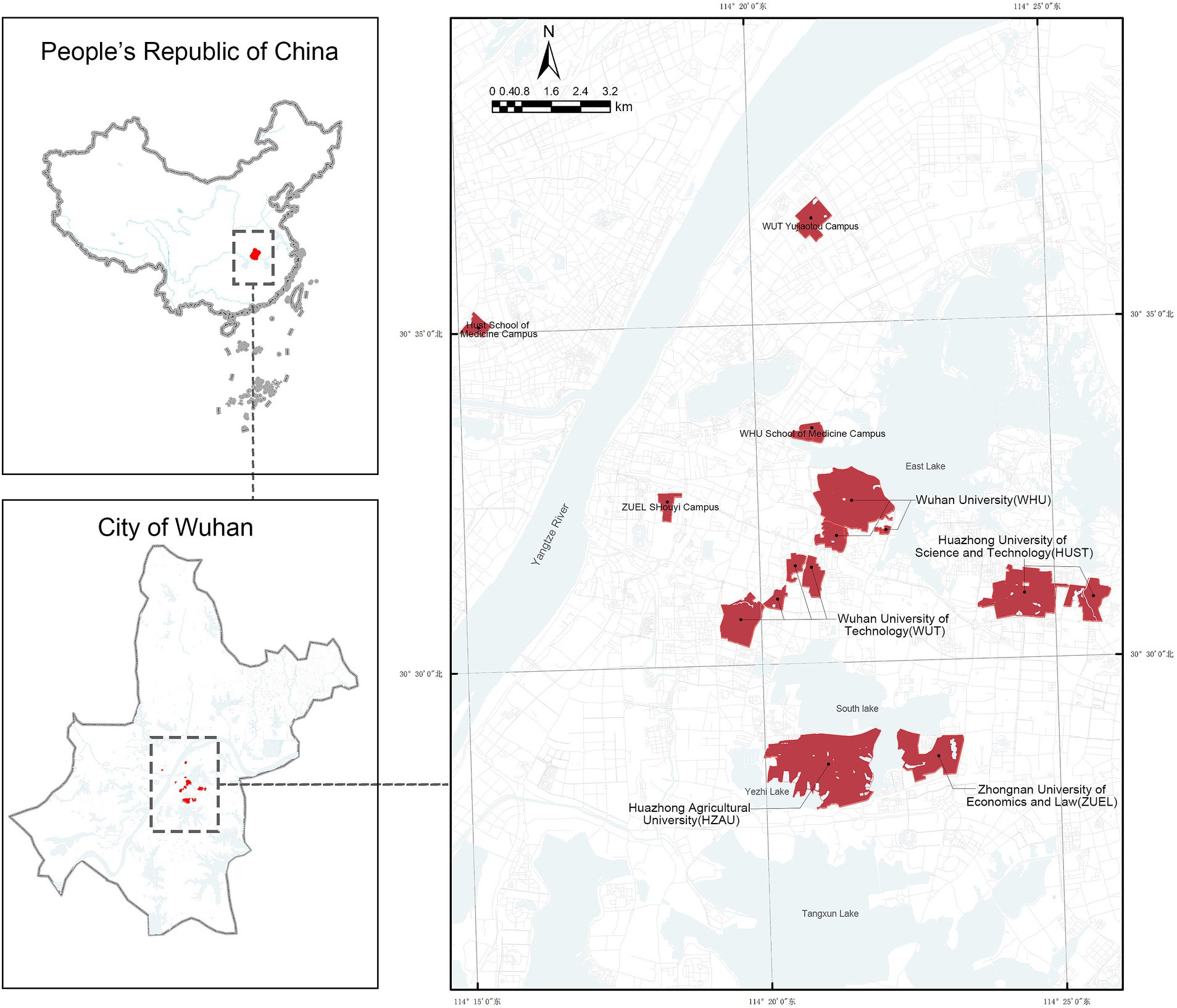
Figure 1. Distribution of the top five largest university campuses in Wuhan.

2.2 Data collection and analysis

The EW data used in this study was obtained from the Dorray fitness application, which categorizes various physical activities and provides key attributes such as spatial location, time, duration, and distance along with walking trajectory data. The study utilized raw walking data collected between 2017 and 2018 for two primary reasons: first, the COVID-19 pandemic significantly restricted walking activities in China from early 2020 through late 2022; second, the two-year period provided a larger dataset, allowing for more robust observations of EW variations.

Data preprocessing was conducted in ArcGIS 10.8. All EW data from the top 5 university campuses in Wuhan was selected, and invalid trajectories caused by anomalies, such as spatial shifts (<1 meter), short activity durations (<1 min), and low speeds (<4 km/h, as defined by the minimum walking speed), were excluded. After cleaning, 5,922 valid trajectories were retained. Following previous research cases (32, 37) and considering the smaller scale of this study, a 50 m × 50 m fishnet grid was created for the 10 campuses using the ArcGIS “Fishnet” tool, overlaying the walking trajectories. This process resulted in 3,557 grids containing EW trajectory data.

Macroscale variables related to satellite-level of campus built environments data, including natural landscapes, urban roads, urban buildings, population density, and land use types, were sourced from the Chinese Resource and Environmental Science Data Center and open-source platforms such as OpenStreetMap. Data on infrastructure and public service points of interest (POI) was gathered from Gaode Maps, while NDVI (Normalized Difference Vegetation Index) data was retrieved from the National Tibetan Plateau Data Center. ArcGIS tools were used to aggregate and process these spatial datasets, and sDNA software was employed to analyze road network data, generating spatial structure indicators. Microscale variables related to eye-level street view data was mostly obtained from Baidu Panorama Map. We used DeepLab V3+ model and ArcGIS to process the streetview data (Figure 2). Processing the street view images, including semantic segmentation and post-processing, required approximately 12 h on a computer with Intel Core i7 CPU and NVIDIA GeForce GTX 1070 GPU. All the data were obtained between June 2017 to May 2018 to minimize temporal discrepancies with the walking trajectory data.

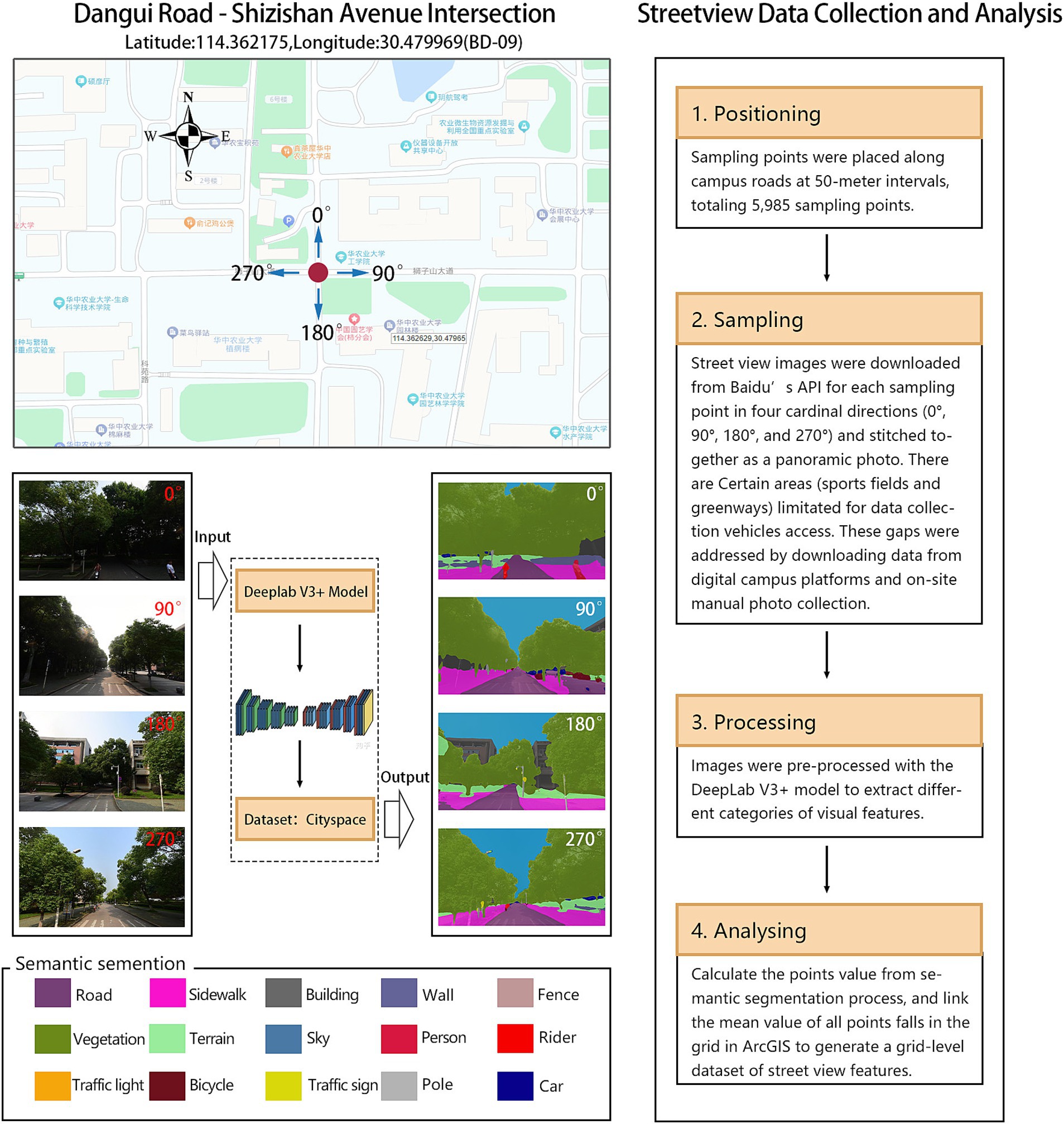
Figure 2. Street view sampling and semantic segmentation with DeepLab V3 + model.

2.3 Variables

Based on previous research on walking indices (38, 39), the EW was calculated as the total number of cleaned walking trajectories within each grid using ArcGIS’s spatial join and data aggregation tools. The EW serves as the dependent variable in this study. Statistical analysis (Table 1) shows that the mean EW is relatively low, indicating a generally low frequency of walking activities within the regions.

Table 1. Descriptive statistics of variables.

The macroscale CBE variables system was constructed using the widely adopted “5D + S” research framework (15, 36). Given the distinct characteristics of campus environments compared to typical urban communities, the variable system integrates modifications from campus-specific walking environment studies (12, 32, 40). At the macroscale level, 21 environmental variables were selected, categorized into five groups: (1) Accessibility to Points of Interest (POI): Distance to public transport facilities (campus parking lots, bus stops) (DT), Distance to fitness or leisure facilities (small sports grounds, gyms, game rooms) (DF), Distance to scenic spots (campus squares, cultural sculptures, pocket parks) (DL), Distance to public service facilities (campus convenience stores, small supermarkets, eyewear shops, photo printing services) (DP), Distance to dining service facilities (restaurants, fast food outlets, bakeries) (DC). (2) Density variables: Building density (BD), Road density (RD), Population density (PD). (3) Building and land use density variables: Residential land use density (RL), Educational and research land use density (TL), Sports land use density (SL), Land use entropy (LE). (4) Spatial network structure variables: Closeness centrality (NQ), Betweenness centrality (BC), Detour ratio (DR), Route efficiency (RE), Block scale (SB). (5) Natural environmental variables: Proximity to water bodies (DW), Green space density (DG), Average slope (SR), Normalized difference vegetation index (NDVI).

At the microscale, six street-level visual factor variables were included based on previous research (20, 41): Green View Index (GVI), Sky View Index (SVI), Vehicular Movement Index (VMI), Visual Humanization Index (VHI), Sidewalk Coverage Ratio (RS), and Shannon Diversity Index (SDI).

The following equations illustrate how some of the variable values in the study are calculated. LE was derived from the Shannon entropy index, which measures the diversity of land use within a region (32). The formula is as follows (Equation 1):

LE=−∑1nPilnPilnn    (1)

where Pi represents the proportion of a specific land use type in the total area. n is the number of land use types.

NQ measures the connectivity of a network by calculating the ratio of network links to the Euclidean distances between an origin point and all accessible destinations within a given radius (32). The formula is as follows (Equation 2):

NQ=∑y∈RxPydMxy    (2)

Where Rx represents the set of links starting from link x within a given network radius. Py represents the weight of node y within the search radius. dM(x,y) is the shortest Euclidean distance from node x to node y (32).

BC is defined as the number of all possible trips through a network link. The formula is as follows (Equation 3):

BC=∑y∈N∑y∈RxPzODyzx    (3)

where ODyzx represents the geodesic distance between endpoints y and z that passes through link x (32).

DR quantifies the degree of detour within a network by calculating the average ratio of geodesic link lengths to crow-fly distances within a given radius. The formula is as follows (Equation 4):

DR=∑y∈RxdMxyCFDxyWyPy∑y∈RxWyPy    (4)

where CFDxy represents the crow-fly distance between the centers of x and y (32, 36).

RE refers to the maximum radius of a convex hull within the network radius, reflecting the maximum spatial coverage of a network’s area (1, 42).

Among Microscale variables, GVI and SVI represent the percentages of vegetation pixels and sky pixels, respectively, in a given image. Both have been shown to significantly influence outdoor physical activity and subjective perceptions (41, 43, 44). The formulas are as follows (Equations 5, 6):

GVI=PgreenPtotal×100%    (5) SVI=PskyPtotal×100%    (6)

where Pgreenrepresents the number of vegetation pixels in the image, Psky represents the number of sky pixels in the image, and Ptotal represents the total number of pixels in the image.

VMI and VHI quantify the degree of motorization and humanization in street spaces, reflecting the dominance of vehicular elements versus pedestrian-friendly features (20, 44). Their formulas are as follows (Equations 7, 8):

VMI=∑1nProad+Ptrafficlight+Ptrafficsign+Pcar    (7) VHI=∑1nPperson+Psidewalk+Prider+Pbike    (8)

where Proad , Ptrafficlight , Ptrafficsign , Pcar represent pixels of roads, traffic lights, traffic signs, and cars in the image; Pperson , Psidewalk , Prider , Pbike represent pixels of pedestrians, sidewalks, riders and bicycles in the image.

RS represents the proportion of sidewalk area relative to the total road surface area, reflecting the quality of street space. Higher RS values are positively associated with walking activities (40, 41). The formula is as follows (Equation 9):

RS=PsidewalkPsidewalk+Proad    (9)

SDI describes the diversity and balance of visual spatial elements. A higher SDI indicates a more diverse and balanced spatial landscape, which has been proven to be both applicable and intuitive (21, 44). The formula is as follows (Equation 10):

SDI=1−∑1nPi2    (10)

where represents the proportion of pixels of element type i relative to the total pixels, and n represents the number of element types. After semantic segmentation, visual features were extracted using the DeepLab V3+ model.

Macroscale and microscale CBE variables were computed and are summarized (Table 1).

2.4 Methods

The workflow of this study is divided into three main steps: First, data collection and variable system development: This step involves collecting and cleaning the data, followed by the establishment of the variable system. Secondly, XGBoost model training and establishing: This step focuses on implementing and training the model. The model training process utilizes several packages in R 4.4.2, including ‘XGBoost’ ‘caret’ ‘shapviz’ ‘shapr’. To address the “black-box” nature of the XGBoost model, SHAP (SHapley Additive exPlanations) was employed to analyze the model’s nonlinear interpretability. Thirdly, Interpretation analysis: This step includes validating the model’s performance and interpreting results such as feature importance (RI), nonlinear correlations, and interaction effects using SHAP. The training and hyperparameter tuning process for all models required approximately 10 h on a computer with Intel Core i7 CPU and NVIDIA GeForce GTX 1070 GPU (Figure 3).

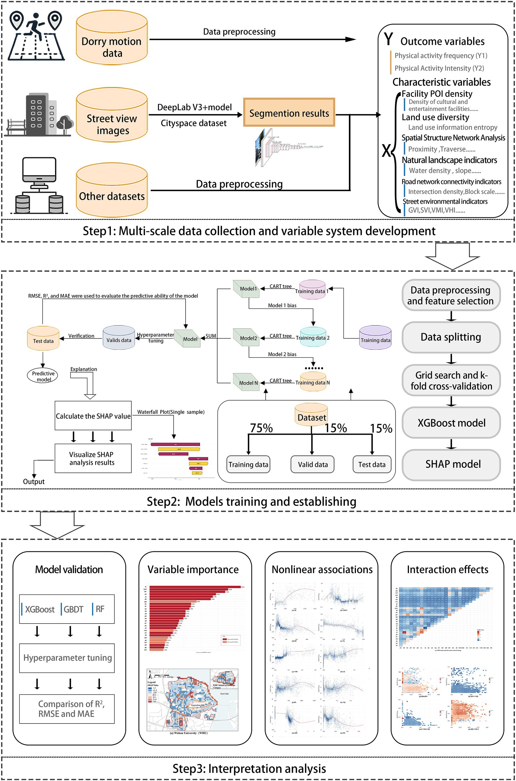
Figure 3. The proposed analytical workflow of the study.

This study employs the Extreme Gradient Boosting (XGBoost) regression tree model to examine the relationship between campus environments and walking activities. XGBoost, introduced by Chen and Guestrin (45), is an optimized distributed gradient boosting library based on Gradient Boosting Decision Trees (GBDT). It is designed for efficient, flexible, and portable machine learning models. By tuning hyperparameters, XGBoost can optimize performance and better explain complex nonlinear relationships among variables (25, 26). GBDT is often compared to another widely used ensemble method, Random Forest. While GBDT is based on the boosting technique, Random Forest employs bagging. In general, although GBDT models are typically more complex and time-consuming, they often outperform Random Forest in terms of accuracy (46).

In this study, we present the key equations of XGBoost to illustrate the theoretical foundation of this model as follows. Additional details can be found in the paper by Chen and Guestrin (45). XGBoost constructs an additive tree-based model where the prediction for each sample is obtained by summing the outputs of K regression trees. The predicted value ŷi is expressed as (Equation 11):

ŷi=∑K=1kfkXi,fk∈F    (11)

where fk represents the k-th tree. The objective function includes a loss term, measuring the difference between true and predicted values, and a regularization term, controlling model complexity. The objective function is defined as (Equation 12):

L=∑i=1nlyiŷi+∑k=1KΩfk    (12)

where lŷiyi represents loss function, measuring the difference between the true and predicted values. Ωfk represents the regularization term, penalizing model complexity to prevent overfitting, defined as (Equation 13):

Ωfk=γΤ+12λ∑j=1Tkwj2    (13)

where Tkrepresents the number of leaves in the k-th tree, wj represents the weight of the j-th leaf, γ represents the penalty parameter controlling the number of leaves, and λ represents the regularization parameter controlling the magnitude of leaf weights.

XGBoost iteratively adds trees to the model using the gradient boosting method. At each iteration t, a new tree is added to minimize the following objective function (Equation 14):

Lt≈∑i=1ngi,ftxi+12hiftxi2+Ωfk    (14)

where gi and hi are the first and second order gradients of the loss function with respect to the predictions. These gradients are defined as (Equations 15, 16):

gi=−∂lyiŷi∂ŷi    (15) hi=−∂2lyiŷi∂ŷi2    (16)

Node splitting is a critical step in tree construction. Splits are determined by maximizing the gain, which measures the improvement in the objective function. Each tree’s structure is determined by potential splits that maximize the gain (Equation 17):

Gain=12GL2HL+λ+GR2HR+λ+GL+GR2HR+HL+λ−γ    (17)

where GL and GR denote sum of first-order gradients for the left and right child nodes, HR and HL denote sum of second-order gradients for the left and right child nodes. The regularization parameter γ and λ can control the complexity of the tree to prevent overfitting.

To interpret the XGBoost model, this study applies SHAP values to interpret the XGBoost model. SHAP values, derived from game theory’s Shapley value concept, are a powerful tool for explaining machine learning model predictions (47). SHAP provides robust, scalable, and interpretable insights, helping to understand the contribution of each feature to model predictions, both globally and locally, particularly valuable for complex “black-box” models like XGBoost and neural networks (48). The SHAP value for a feature i is expressed as follows (Equation 18):

ϕi=∑S⊆N\i|S|!|N|−|S|−1!|N|!fS∪i−fS    (18)

where ϕi represents the contribution of feature i, N represents the set of all p features, fS∪i and fS represents model prediction with and without feature i, respectively. The SHAP value ϕi can be positive, negative, or zero, representing whether the feature increases, decreases, or does not affect the prediction, respectively. The absolute SHAP value reflects the magnitude of the feature’s impact on the model’s output. The relative importance of a feature is calculated as the average of its absolute SHAP values (Equation 19):

fx=ϕ0+∑i=1Mϕi    (19)

where M represents number of input features, ϕ0 represents base value of the model output, and ϕi represents Shapley value for feature i. This approach allows for interpreting the contributions of individual features and understanding the nonlinear effects within the XGBoost model.

3 Results 3.1 Model validation

To validate the model more effectively, we compared the performance of three different machine learning models: the XGBoost, the GBDT, and the Random Forest regression model. To ensure consistency in experimental conditions, we first examined multicollinearity among the independent variables and removed variables with a Variance Inflation Factor (VIF) greater than 10 (20, 49, 50). Given our objective to compare model performance rather than deploy models on new data, and considering the relatively small sample size (3,557 grids), we divided the dataset into 80% training and 20% validation data. To analyze the data distribution of different variables across various datasets, we conducted a comprehensive assessment using the Kolmogorov–Smirnov (KS) test and histogram plots. The analytical results are available in the Supplementary materials. Our analysis revealed that most variables exhibited consistent distributions across datasets. However, the dependent variable (WE) showed skewness. To address this and improve data quality, we applied preprocessing techniques, including square root transformation and standardization, prior to conducting hyperparameter tuning.

To enhance model performance and mitigate overfitting, this study employed Bayesian optimization for systematic hyperparameter tuning of the XGBoost model. Bayesian optimization efficiently identifies optimal combinations of hyperparameters by leveraging a probabilistic model to guide the search process, focusing on promising regions of the hyperparameter space while minimizing the number of evaluations (51). Additionally, 5-fold cross-validation was utilized to ensure the robustness of the model. For reproducibility, key hyperparameters were optimized within the following ranges: learning rate (eta: 0.01–0.05) to control iteration step size; tree depth (max_depth: 6–10) for model complexity and nonlinear relationships; sample ratio (subsample: 0.6–0.9) to reduce overfitting by selecting subsets of training samples; feature sampling ratio (colsample_bytree: 0.6–0.9) for features per tree; minimum leaf weight (min_child_weight: 10–30) to enhance robustness; minimum split loss (gamma: 0–5) to prevent excessive splitting; and L2 (lambda) and L1 (alpha) regularization (1–20) to limit model complexity.

The optimization began with 10 initial points to construct the surrogate model, followed by 60 iterations to identify the optimal parameters. A similar preprocessing and tuning strategy was applied for GBDT and Random Forest, enabling a comparative analysis of predictive performance. The best XGBoost parameters were determined as follows: eta: 0.0328, max_depth: 10, subsample: 0.9, colsample_bytree: 0.7862, min_child_weight: 10, minimum split loss: 0, lambda: 20, alpha: 5.

The machine learning model’s performance is assessed primarily by its predictive power, which is commonly evaluated using three key metrics (20, 24): Coefficient of Determination (R2): Measures the goodness of fit for statistical models with values ranging from 0 to 1; higher values indicate better predictive accuracy. Root Mean Squared Error (RMSE): Represents the square root of the mean squared differences between predicted and actual values, with smaller values indicating better accuracy. Mean Absolute Error (MAE): The average of the absolute differences between predicted and actual values, with smaller values indicating higher precision.

The results (Table 2) highlight the core parameter metrics and performance of the three models. They indicate that the XGBoost model achieved a relatively higher R2 value than the other two models, while its RMSE and MAE values were lower. These findings demonstrate that the XGBoost model outperformed the GBDT and Random Forest models in this study, highlighting its enhanced capability to address nonlinear regression problems (46).

Table 2. Model parameters and performance evaluation.

3.2 RI

The relative importance (RI) of independent variables was measured using the average absolute SHAP values, which reflect the extent to which each feature influences the model’s output. After calculating the mean absolute SHAP values for all features, the variables were ranked from highest to lowest. The analysis was visualized using bar plots, beeswarm plots, and ArcGIS maps (Figures 4, 5) (47).

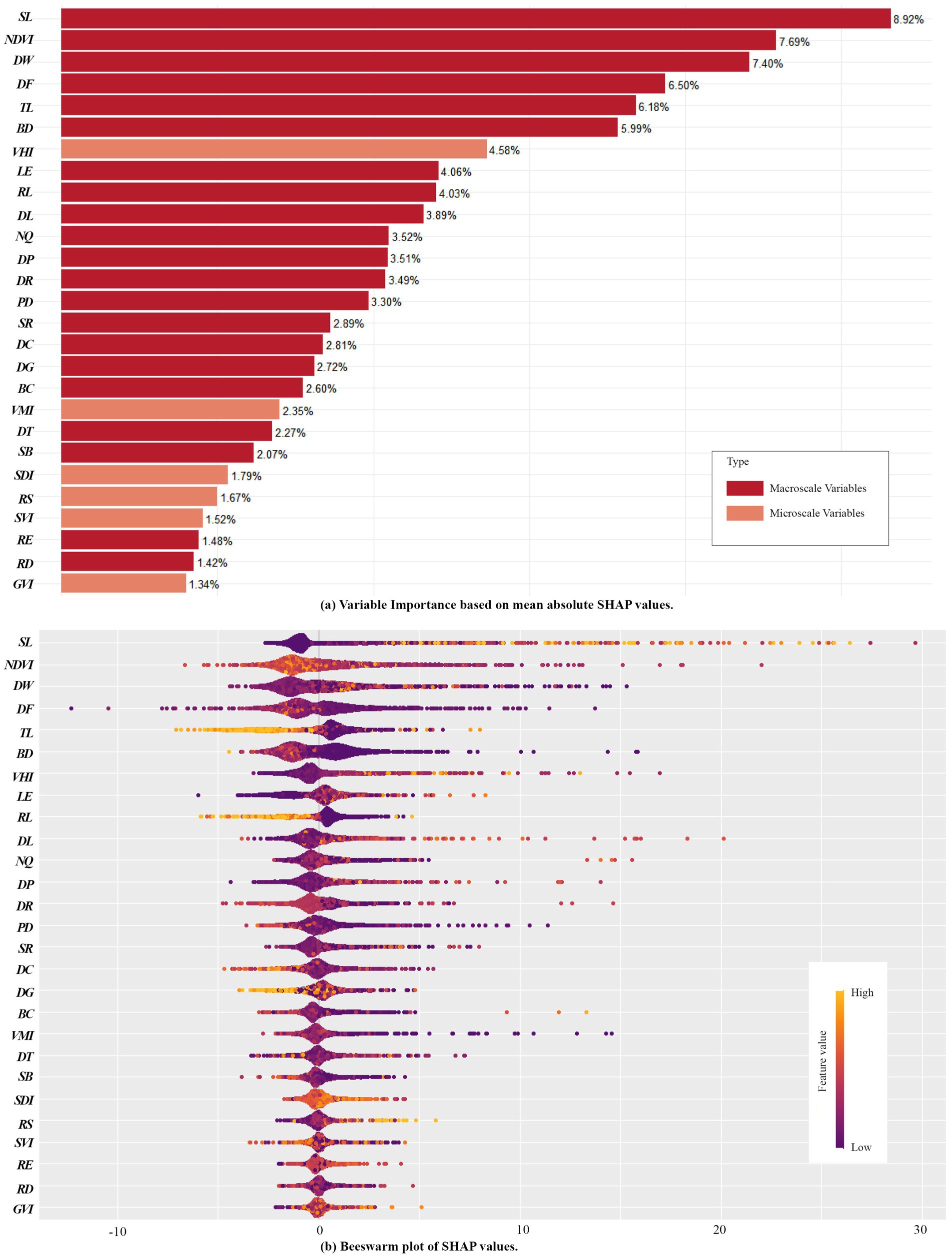
Figure 4. RI of Variables derived using the SHAP model. (a) Variable Importance based on mean absolute SHAP values; (b) Beeswarm plots of SHAP values.

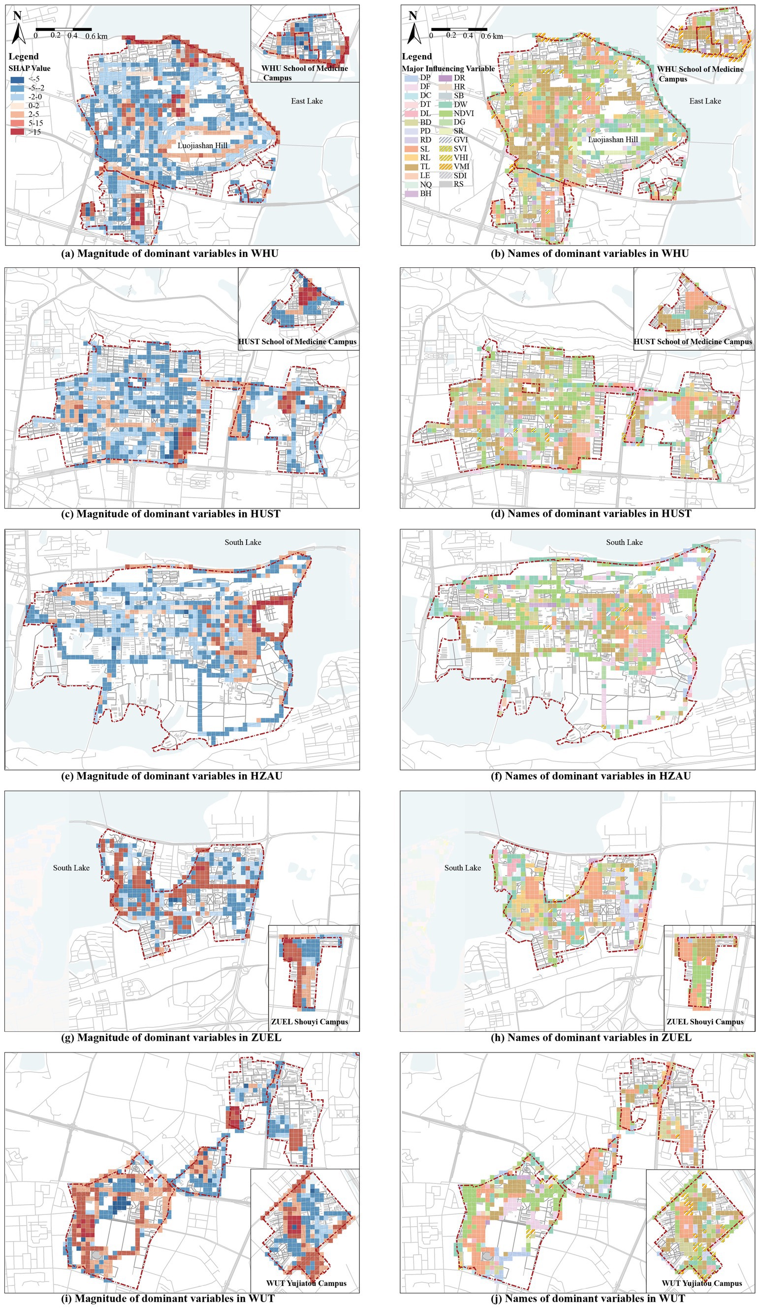
Figure 5. Distribution of dominant factors of local impacts obtained from the SHAP model. (a) Magnitude of dominant variables in WHU; (b) Names of dominant variables in WHU; (c) Magnitude of dominant variables in HUST; (d) Names of dominant variables in HUST; (e) Magnitude of dominant variables in HZAU; (f) Names of dominant variables in HZAU; (g) Magnitude of dominant variables in ZUEL; (h) Names of dominant variables in ZUEL; (i) Magnitude of dominant variables in WUT; (j) Names of dominant variables in WUT.

The relative contribution of macroscale CBE variables and microscale CBE variables to EW is 86.75 and 13.25%, respectively. This indicates that macroscale built environments variables within campuses play a dominant role in influencing exercise walking (Figure 4A). The top-ranking independent variables in terms of RI are in order, SL (8.92%), NDVI (7.69%), DW (7.40%), DF (6.50%), TL (6.18%), BD (5.99%), VHI (4.58%), LE (4.06%), RL (4.03%), DL (3.89%), NQ (3.52%), DP (3.51%), DR (3.49%), PD (3.30%), and the influence of other variables accounted for less than 3%. Among them, the influence of sports land use density is the most significant, indicating that the quantity and accessibility of sports facilities are closely linked to campus walking activities. This is consistent with previous research findings (32, 40). Similar to findings in park environments, beautiful natural landscapes and aesthetic human-made features significantly enhance walking activities (40, 52), likely due to the scenic and recreational appeal of natural features, which improves the walking experience. Particularly, Wuhan’s University campuses, with their proximity to water bodies, demonstrate strong positive impacts on walking activities, consistent with recent studies highlighting the positive effects of urban water environments on physical activity (53). The influence of residential land use proportion, educational and research land use proportion, building density, and land use diversity further supports their critical role in influencing EW within campus environments (32, 54).

Notably, CBE variables related to spatial structure and road connectivity, such as road density, route efficiency, block scale, and betweenness centrality, exhibit relatively weak influence. Similarly, DG does not show significant impact. These findings are inconsistent with current studies on urban environments, where such factors are often prominent influencers of physical activity (54–56). This divergence may stem from the low building density and distinct functional zoning within campuses, as well as differing purposes of walking activities (e.g., commuting vs. exercise walking).

Beeswarm plots illustrate the distribution of SHAP values across samples where wider areas represent a high concentration of samples, while longer extensions on the right or left indicate stronger positive or negative contributions to SHAP values, respectively. Redder hues represent higher feature values, while bluer hues represent lower values (57). From Figure 4B, variables such as SL VHI, and RS exhibit positive correlations with exercise walking. Conversely, RL, TL, and BD display negative correlations. Other variables exhibit less distinct patterns, suggesting potential complex nonlinear relationships.

To clarify spatial heterogeneity of campus CBE and provides insights into the localized impacts of different environmental features on EW, we calculated the dominant influencing variables for each sample of the SHAP model. These dominant variable values were assigned to each grid, and local explanation maps were generated in ArcGIS to visualize the influence of campus environments on exercise walking (Figure 5). Figures 5A, C, E, G, I show the magnitude of dominant variables. Red represents positive impacts on EW, while blue indicates negative impacts, with deeper colors signifying stronger effects. Figures 5B, D, F, H, J annotate the names of the dominant influencing variables.

The high-impact areas across the five university campuses align with the RI rankings are concentrated in the following six typical regions:

(1) Sports fields: All five university campuses exhibit strong positive impacts in campus sports field areas. The dominant variable in these regions is the SL and its influencing areas often spills over into adjacent grids.

(2) Residential and educational zones: Large residential and science and education zones within all campuses generally have negative impacts on exercise walking. The dominant variables in these areas are RL and TL and some grids are also influenced by BD and other variables.

(3) Proximity to large water bodies: The Lakeside campus exhibit a significant positive impact in their peripheral areas along the lakes. For instance, grids near Donghu Lake at WHU, and Nanhu Lake near HZAU and ZUEL, show strong positive impacts. The dominant variable in these areas is mostly DW, with some influence from NDVI and other factors.

(4) Major boulevards of larger campus and connecting roads between campuses: In larger campuses, the boulevard has a strong positive influence on EW in surrounding grids, such as Shizishan Boulevard at HZAU, Zhongnan Boulevard at ZUEL, and Zijing Road at HUST. These roads typically feature large trees along both sides, wide pedestrian areas, less vehicular traffic, and open sight lines. Similarly, the connecting roads between multiple campuses also show strong positive effects, such as Bayi Road between the north and south campuses of WHU, and Yuyuan Road between the east and west campuses of HUST. As major transport routes linking key functional areas within and between campuses, these roads experience higher pedestrian flows, which is reasonable. The dominant influencing factors along these roads are also more diverse.

(5) Areas Along smaller campus gates: Areas such as the southern side of WHU’s Medical School, the western side of HUST’s East Campus, and the southeastern side of WUT’s Yujiatou Campus have dominant grids influenced by VMI and VHI. These areas, located at the campus-urban interface, experience relatively high urban vitality, which positively impacts exercise walking (32, 41). In smaller campuses, the proximity to campus gates enhances accessibility and efficiency, leading to a more noticeable influence from the surrounding urban environment. This makes the areas around these gates particularly significant in shaping walking patterns.

(6) Circular Paths and Greenways: Some circular road grids within WHU, HZAU, and WUT campuses show continuous positive effects. The representative one is the forest trail around Luojia Mountain at WHU, where the most dominant variable is NDVI. Similar high-impact circular roads in campuses like HZAU and WUT, such as greenways and secondary roads, exhibit diverse dominant variables. Circular paths provide a scenic, safe, and comfortable environment for walkers, enriching the walking experience and enhancing their appeal for exercise walking (22,