Subjects

The analysis of 18F-DOPA uptake in the striatum has already been published for this dataset (for both the saline- and ketamine-treated animals and the test–retest cohort) [8]. These scans were re-analysed here to assess 18F-DOPA uptake in the midbrain, and therefore no new animals were used for this study. The details below refer to the original cohorts of animals. Wild-type male C57BL/6J mice were acquired from Charles River (Kent, UK). Animals were housed in groups of up to 4 and provided with ad libitum food and water. Animals were acclimatised to the facility for at least 1 week prior to any experimental procedures, which were undertaken in adult animals (8–12 weeks old). For animal weights, see Table 1. All animal experimental procedures were performed in accordance with the UK Animals (Scientific Procedures) Act 1986 and EU directive 2010/63/EU, and protocols were approved by the Imperial College Animal Welfare and Ethical Review Body and conducted under the licence PE0206466.

Table 1 Animal weights and injected 18F-DOPA dose for the saline and ketamine-treated cohorts, and the test–retest cohort. Mean (SD)Experimental CohortsSaline-Treated Cohort

Animals were administered saline intraperitoneally (i.p.; 0.9%) once daily for 5 consecutive days, as they formed the control cohort for the ketamine treatment (see below). Animals then underwent the PET scan on day 7. Animals were euthanized immediately after the scan. Although 14 animals were originally treated with saline, 2 animals were excluded from analysis due to issues with the scan data, resulting in a final n = 12 for this group. This cohort was used to establish the midbrain template and the analysis parameters which resulted in the best-fitting data and lowest intra-group variability when estimating 18F-DOPA uptake in the midbrain.

Ketamine-Treated Cohort

To generate the sub-chronic ketamine model, ketamine hydrochloride (Sigma-Aldrich, K2753) was dissolved in 0.9% saline solution and administered to mice (n = 12) at a dose of 30 mg/kg (i.p) once daily for 5 consecutive days. On day 7, after 2 days of washout, animals underwent an 18F-DOPA preclinical PET scan. Animals were euthanized immediately after the scan.

Test-Retest Cohort

A separate cohort of untreated mice (n = 6) was scanned twice to assess reproducibility of results. Animals underwent the initial scan (“test”) and were then recovered from the anaesthesia. They were re-scanned (“retest”) approximately 48 h later, after which they were immediately euthanized.

PET Acquisition

18F-DOPA was synthesised as described previously [19]. One hour prior to the administration of 18F-DOPA, mice were anaesthetised with isoflurane (4%), which was maintained at 1–2% for the duration of the scan (O2 1 L/min). Respiration rate and body temperature were continuously monitored (BioVet, m2m Imaging Corp, OH, USA). To prevent peripheral metabolism of 18F-DOPA, inhibitors of catechol-O-methyl-transferase (COMT) and aromatic amino acid decarboxylase (AADC)—entacapone (40 mg/kg; Sigma-Aldrich, SML0654) and benserazide hydrochloride (10 mg/kg; Sigma-Aldrich, B7283)—were given i.p. 45 min and 30 min prior to the administration of 18F-DOPA, respectively [6, 17, 20]. To avoid competition with the uptake of other neutral amino acids in the diet, animals were fasted for 45 min before being anaesthetised [6, 21]. An i.p. cannula used to deliver the radiotracer was inserted 30 min prior to the scan. The mice were then placed into an Inveon PET/CT scanner (Siemens, Surrey, UK) and underwent a 10-min CT scan to allow for attenuation correction of the PET signal. A dynamic PET scan was then started concomitantly with the delivery of 18F-DOPA via the i.p. cannula, and data were collected for 140 min. The test–retest datasets were only acquired up to 120 min, due to changes in the scanning parameters between cohorts. The average 18F-DOPA doses delivered for each experimental cohort are provided in Table 1.

PET Image Processing

Following acquisition, data were histogrammed into 45 frames (10 × 3 s, 6 × 5 s, 8 × 30 s, 5 × 60 s, 6 × 300 s, 8 × 600s for data acquired up to 120 min). For data acquired up to 140 min, an additional 2 × 600 s frames were added. Data were reconstructed using filtered back projection with CT attenuation correction, adjusting for random noise, scatter, and radiotracer decay. Image processing was carried out using the Inveon Research Workspace software (Siemens, USA). The CT image was manually co-registered to the reconstructed PET image using the outline of the skull as a reference. For each subject, the percentage-injected dose was normalised for body weight and injected activity to provide standardised uptake values (SUV). The striatal (0.70 mm3) and cerebellar (the reference region; rectangular; 1.1 mm3) regions of interest (ROI) were placed manually on summation radioactivity images guided by CT and mouse brain anatomy based on previous studies [6, 8, 17].

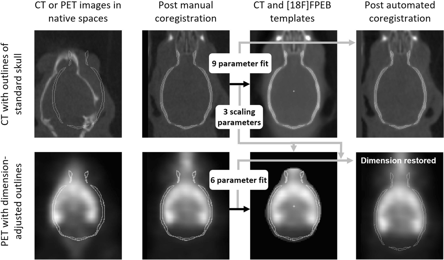
Developing the Midbrain Template

Based on stereotaxic coordinates from the Paxinos Mouse Brain Atlas, the volume of the midbrain region which incorporates the bilateral SNpc and VTA is approximately 3.2 mm3 [22] (Supp. Figure S1a). Therefore, we established a rectangular midbrain ROI of 3.7 mm3 (16 voxels, Supp. Table S1). A template was developed to standardise the placement of this ROI in the brain; a representative CT image at the midline sagittal viewpoint was aligned with a mask based on the sagittal P56 Allen Mouse Brain Atlas, image 21 (mouse.brain-map.org/static/atlas [23]) to identify the location of the midbrain (Fig. 1). The resulting template was applied to the CT images of each animal to place the midbrain ROI. Supplementary figure S1b shows the placements for all 12 saline-treated animals.

Fig. 1

Developing the midbrain template. a An atlas image of the mousebrain sagittal midline (from the Allen Mouse Brain Atlas) was used to identify the midbrain region, and a mask based on this atlas image (green) was aligned to an ROI drawn within the outline of the skull from a representative mouse CT scan. The cerebellum (yellow) was placed in the posterior part of the brain. This template was then used to place the 3.7-mm3 midbrain ROI (blue), seen from the b coronal and c sagittal perspective. The 18F-DOPA signal (yellow-red spectrum) can be seen in the d coronal and e sagittal planes, along with the placement of the midbrain ROI

Modified Patlak Analysis

The kinetic analysis to provide an estimate of the rate of 18F-DOPA uptake was performed using a MATLAB pipeline developed in-house (version R2022a; MathWorks, MA, USA). A modified Patlak graphical analysis was used to determine the influx rate constant KiMod (min−1). KiMod is a modified version of the influx rate constant KiStd (min−1) and takes into account an estimation of kloss (min−1), the rate at which signal is removed from the system due to metabolism of 18F-dopamine, as described previously [20, 24,25,26]. To establish the optimal time window for estimating KiMod in the midbrain, data from the saline-treated animals were processed through the modified Patlak analysis pipeline using varying start (T*) and end times (Tend). The analysis pipeline also quantifies the coefficient of variation (CV%) for the Patlak modelling, which gives an indication of how well the fitting has worked. These numbers were also compared for each T*–Tend window, with the lowest CV% indicating the best fit of the data to the graphical model. In some instances, the Patlak model can fail due to excessive noise in the data, or too few usable data points. This requires these datasets to be excluded, and therefore the number of animals included for each T*–Tend window (as a fraction of the whole group) is also noted.

Statistical Analysis

Statistical tests were carried out using GraphPad Prism v9 (GraphPad Software, La Jolla, California, USA). Data were tested for statistical outliers (Grubbs, α = 0.05) and normality (Kolmogorov-Smirnov test). Significance was defined as α < 0.05. Data is always presented as mean ± standard deviation (SD). SD of the saline-treated cohort was compared for each T*–Tend time windows to determine the parameters which produced the least within-group variability. T-test was used to compare mean differences between groups, with Welch’s correction used where variance was significantly different between groups. Consistency between the test–retest scans was analysed using an intra-class correlation coefficient (ICC; using a two-way mixed model with absolute agreement) and absolute percentage variance (%). Pearson’s correlations coefficients were calculated to assess significant linear correlations.